Exploring Model Quantization for LLMs

May 1, 2024

LLaMAllama.cppGGUFGPTQAWQ

What is Model Quantization?

At its core, model quantization is all about efficiency. Imagine you’ve got a super heavy textbook (like one of those old school encyclopedias) that you need to carry around all day. Pretty exhausting, right? Now, what if you could shrink that down to the size of a comic book, while keeping all the essential info intact? That’s essentially what quantization does to LLMs: it compresses their size without losing the essence of what they can do.

In technical terms, quantization reduces the precision of the numbers (weights) used in a model from full floating-point to half fp, N bit fp or integers. This doesn’t just make the model lighter but also speeds up its calculations, because crunching smaller numbers takes less work for computers.

FP32, FP16, BFP16:

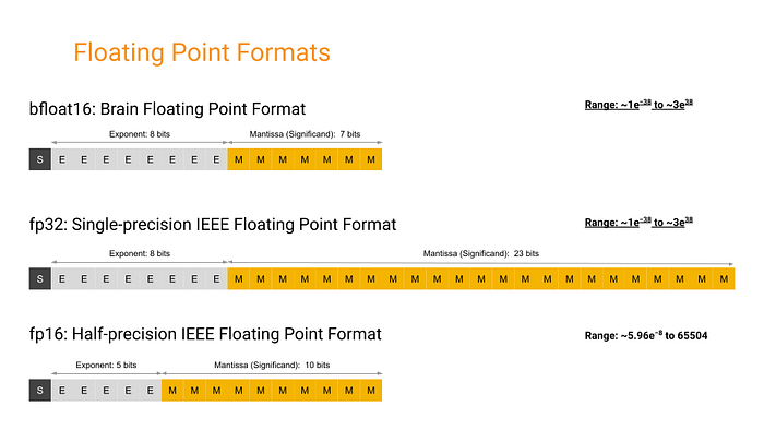FP32 vs FP16 vs BFP16 precision comparison Source: Google

Benefits of Model Quantization

Reduced Model Size: Quantized models take up less space. This means we can run our LLMs on devices with less memory: think MacBook Air, smartphones, IoT devices, and even on the edge (like in your smart fridge!).
Increased Performance: With smaller data sizes, quantized models can operate faster, making them ideal for applications that require real-time processing. This is crucial for features like instant recommendations.
Broader Deployment Possibilities: Because these models are smaller and faster, they can be deployed in environments where computing power is limited. This opens up a whole new world where advanced AI can be used in places we never thought possible.

Quantization lets us do more with less, making LLMs both more accessible and more sustainable.

Key Quantization Formats and Techniques

GGML (Georgi Gerganov Model Language)

Developed by Georgi Gerganov, GGML was a pioneer, simplifying model sharing by bundling everything into a single file. Think of it as the cassette tape 📼 of model formats: straightforward and widely compatible with different CPUs. It facilitated model sharing and execution, including those in Apple Silicon devices.

GGUF (GPT-Generated Unified Format)

Then came GGUF, like the DVD 📀 of formats. Introduced on August 21, 2023 (GGML officially phased out, new format called GGUF #1370), GGUF brought enhanced flexibility and compatibility, supporting a broader range of models and features. It retained the qualities of GGML while adding backward compatibility and extended support across various model types, including Meta’s LLaMA.

GPTQ (Generative Post Training Quantization)

GPTQ is like the Blu-ray 🥏 in our story: it emerged to address the need for highly efficient post-training quantization to compress models significantly while maintaining high accuracy, especially useful for GPUs.

GPTQ reduces the bit representation of model weights post-training, compressing model size significantly while retaining performance integrity.
By reducing the bit-depth of weights from standard floating points to just 3–4 bits, GPTQ allows models to consume significantly less memory: up to 4x less than FP16 models.
Unlike FP16, GPTQ’s aggressive compression strategies make it suitable for memory-constrained environments without a substantial compromise on performance.

K-quants

The K-quant approach is a bit like having different resolution settings in video 🎞️: much like a photographer adjusts the focus on various parts of a scene, emphasizing details where they matter most. It adjusts the precision for different parts of the model, balancing performance and detail based on the computational budget.

Block-based weight division: Model weights are segmented into blocks, where each block can have a different quantization precision based on its importance or impact on model performance.
Selective precision application: This method allows for finer control over which parts of the model are compressed more heavily, optimizing both performance and size effectively.

EXL2

EXL2 focuses on maximizing GPU utilization: think of it as the 4K Ultra HD 📷 of quantization, providing high efficiency and precision, primarily geared for newer GPUs.

VRAM utilization: EXL2 optimizes VRAM usage, enabling larger models to run on GPUs that would otherwise not handle them.
Inference speed: Particularly on newer GPU hardware, EXL2 delivers faster inference times by reducing the computational overhead required to process the quantized weights.

AWQ (Activation-Aware Weight Quantization)

AWQ takes a unique approach by quantizing weights based on their activation during inference, protecting the most critical weights to minimize performance loss. It’s like a skilled chef 🧑‍🍳 treats ingredients: carefully measuring and optimizing each component for the perfect balance!

AWQ considers how each weight impacts the model’s activations during actual data processing, quantizing more aggressively where the impact on output quality is minimal.
This allows AWQ to maintain or even enhance model performance by preserving the fidelity of activations where it counts most.

QAT (Quantization-Aware Training)

QAT is like training an athlete 🏃🏻‍♂️ with the gear they’ll use on race day: ensuring peak performance under quantization constraints. It integrates quantization into the training process itself, ensuring the model performs well even at reduced precision.

QAT embeds quantization directly into the model training cycle, allowing the model to adapt to quantization-induced nuances from the start.
By training with quantization in mind, QAT produces models that are inherently more robust and accurate under quantized conditions, avoiding the performance drop typically seen with post-training quantization.

PTQ (Post-Training Quantization)

PTQ is like adding a turbocharger to a car engine: applied after the model is fully trained to tweak performance without extensive retraining, perfect for quick deployments.

Relatively easy to implement, requiring minimal changes to the existing model structure.
Widely used when there’s a need for rapid deployment or when retraining with QAT isn’t feasible due to resource constraints.

In summary…

The evolution from GGML to GGUF, GPTQ, and EXL2 showcases significant technological advancements in model compression. GGML simplified model sharing with CPU-compatible single-file bundles. GGUF added backward compatibility and broader model support. GPTQ introduced aggressive GPU-optimized compression with minimal performance trade-off. K-quants brought selective precision management to balance performance and size. EXL2 pushed GPU efficiency to the limit: maximizing inference speed and enabling larger models on modern hardware.

Strengths, Limitations, and Best Applications

GGML vs. GGUF

Advantages

GGML: Simple, CPU-friendly, good for initial deployments on diverse platforms including Apple Silicon.
GGUF: Offers backward compatibility, supports a wider range of models, and integrates additional metadata directly.

Limitations

GGML: Struggles with flexibility and compatibility with newer model features.
GGUF: Transitioning existing models to GGUF can be time-consuming.

Best Use Scenarios

GGML: Best for straightforward model deployment across basic computational setups.
GGUF: Ideal for more complex models requiring ongoing updates and backward compatibility.

GPTQ

Advantages

Highly efficient memory usage, reducing model size significantly without severely impacting performance.
Suitable for environments where GPU memory is limited.

Limitations

May incur some accuracy loss due to the aggressive compression.

Best Use Scenarios

Perfect for GPU-constrained environments where maintaining a balance between performance and memory usage is crucial.

K-quants

Advantages

Allows selective precision application, optimizing performance where it counts.
Adjusts quantization depth dynamically based on the importance of different model parts.

Limitations

More complex to implement due to the need for determining the importance of different model components.

Best Use Scenarios

Great for applications where specific model components play critical roles, such as detailed image or speech processing tasks.

EXL2

Advantages

Optimizes VRAM usage, allowing larger models to run on newer GPU hardware.
Enhances inference speed significantly.

Limitations

Perceived as more complex and less user-friendly compared to GGUF.
Less community support and fewer available models, limiting visibility and adoption.

Best Use Scenarios

Best suited for cutting-edge GPU environments where maximum inference speed and model size optimization are required.

AWQ

Advantages

Focuses on preserving the quality of activations, minimizing the impact on model performance.
Adapts quantization levels based on activation importance.

Limitations

Requires initial data-driven calibration, which can be data-intensive.

Best Use Scenarios

Ideal for scenarios where model accuracy is paramount and sufficient calibration data is available.

QAT vs PTQ

Advantages

QAT: Integrates quantization into the training process, producing models that are robust to quantization effects.
PTQ: Easier to apply: no changes to the training process, suitable for quick deployments.

Limitations

QAT: Time-consuming and computationally expensive.
PTQ: May lead to a performance drop if not carefully managed.

Best Use Scenarios

QAT: Best when developing a new model from scratch with quantization in mind.
PTQ: Suitable for rapid deployment of existing pre-trained models.

Model suitability and deployment environments

For legacy systems or limited computing power: GGML and PTQ offer straightforward solutions.
High-performance GPU environments: EXL2 and GPTQ optimize the trade-off between performance and memory.
Accuracy-critical applications: AWQ and QAT are preferred when the deployment environment can handle the associated overhead.

Quantized Model Files

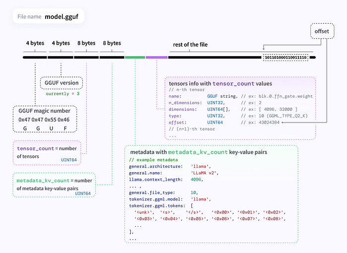GGUF file format diagram diagram by @mishig25 (GGUF v3)

Finding GGUF files

Browse all models with GGUF files by filtering with the GGUF tag: hf.co/models?library=gguf
Use the ggml-org/gguf-my-repo tool to convert/quantize your model weights into GGUF format.

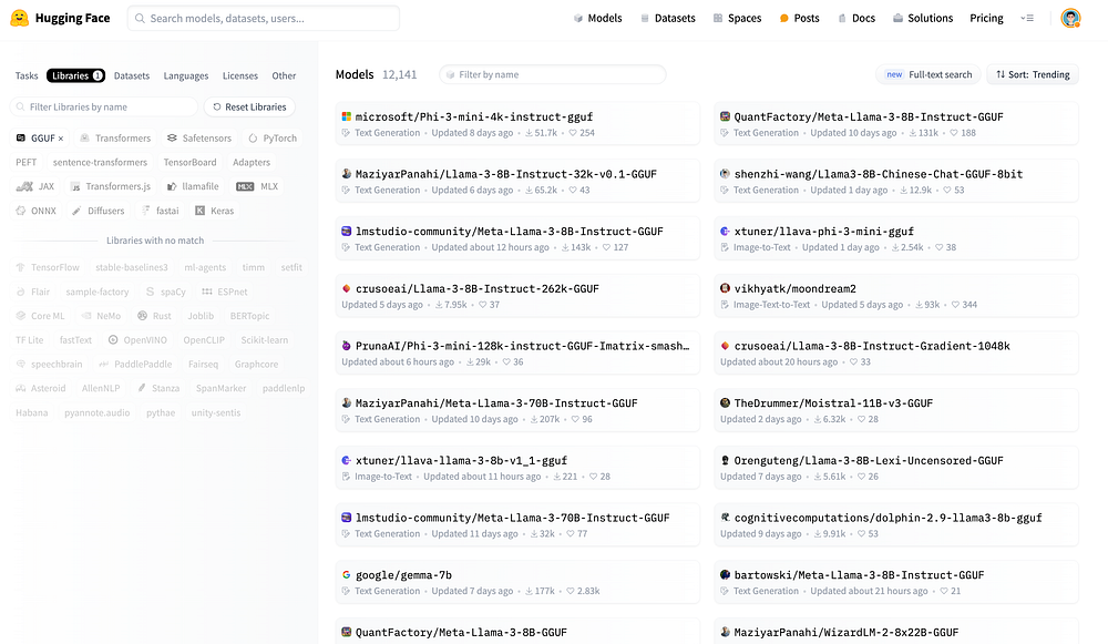HuggingFace Model Hub

Quantization Types

What are these different GGUF files?

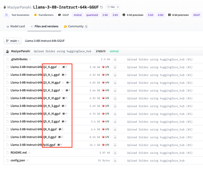Different Model Quantization Files

Here’s a breakdown of what each part of the filename means:

Q(Number): The “Q” followed by a number (e.g., Q2, Q3, Q4) refers to the bit depth of quantization. Lower bit quantizations like Q2 are more aggressive: smaller model sizes but potentially higher quality loss. Higher bit depths like Q6 provide less compression, maintaining better fidelity at the cost of larger sizes.
K: The _K suffix (like Q4_K, Q5_K) indicates specific optimizations within the quantization framework: often targeting certain layers to minimize quality loss.
S, M, L: Stand for Small, Medium, and Large: different balances between model size and accuracy:
- S (Small): Lowest memory usage, highest compression.
- M (Medium): Balanced memory usage and performance.
- L (Large): Higher accuracy at the cost of more memory.

Practical usage

Consider your hardware (RAM and VRAM) and your performance vs. accuracy requirements:

Limited VRAM but need fast performance → Q5_K_S
Can afford more memory and need higher accuracy → Q5_K_L

For Apple Silicon with M1 and 16GB RAM:

Q5_K_M (4.45GB for 7B): Very low quality loss, one of the more balanced options.
Q3_K_M (3.06GB for 7B): Good balance between memory and perplexity increase; more suitable if RAM is a hard constraint.

For an Nvidia GPU with 16GB VRAM:

Q6_K (5.15GB for 7B): Excellent for high-performance needs with minimal quality loss.
Q5_K_M (4.45GB for 7B): Good balance between model size and perplexity increase.

The Hub has a viewer for GGUF files that lets you inspect metadata and tensor info (name, shape, precision).

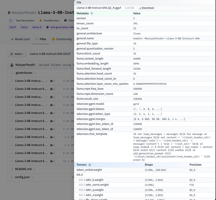GGUF file details on HuggingFace

How to Load and Run Quantized Models

llama.cpp

llama.cpp is a C/C++ LLM inference framework optimized for efficient CPU inference, especially for the Meta Llama architecture. It integrates with Cosmopolitan Libc to provide a cross-platform solution that runs across operating systems without recompilation.

Cosmopolitan Libc makes C a build-once run-anywhere language, like Java, except it doesn’t need an interpreter or virtual machine. Instead, it reconfigures stock GCC and Clang to output a POSIX-approved polyglot format that runs natively on Linux + Mac + Windows + FreeBSD + OpenBSD + NetBSD + BIOS with the best possible performance and the tiniest footprint imaginable.

Installation on Apple Silicon

Full documentation: docs/install/macos.md

pip uninstall llama-cpp-python -y
CMAKE_ARGS="-DLLAMA_BLAS=ON -DLLAMA_BLAS_VENDOR=OpenBLAS -DLLAMA_METAL=on" \
pip install llama-cpp-python \
--upgrade --force-reinstall --no-cache-dir

Installation on Nvidia GPU

CUDACXX=/usr/local/cuda-12/bin/nvcc \
CMAKE_ARGS="-DLLAMA_CUBLAS=on -DCMAKE_CUDA_ARCHITECTURES=native" \
FORCE_CMAKE=1 \
pip install llama-cpp-python \
--no-cache-dir --force-reinstall --upgrade

Code example

import platform
from llama_cpp import Llama
from IPython.display import Markdown, display

print(platform.platform())
# macOS-14.4.1-arm64-arm-64bit

# Load local model
llm = Llama(
    model_path="sanctumAI-meta-llama-3-8b-instruct.Q4_K_S.gguf",
    n_ctx=8192,
    vocab_only=False,
    use_mmap=True,
    use_mlock=False,
    n_gpu_layers=-1,
    split_mode=llama_cpp.LLAMA_SPLIT_MODE_ROW,
    n_threads=5,
    verbose=True,
)

SYSTEM_PROMPT = (
    'You are a helpful assistant that helps users with their queries. '
    'You are expected to provide accurate and relevant information to the user.'
)

QUERY = "How can I generate a requirements.txt file with all the python packages installed in local environment?"

response = llm.create_chat_completion(
    messages=[
        {"role": "system", "content": SYSTEM_PROMPT},
        {"role": "user", "content": QUERY}
    ],
    max_tokens=512,
    temperature=0.7,
    top_p=0.95,
    stop=["[/INST]"]
)

display(Markdown(response['choices'][0]['message']['content']))

llama_print_timings:        load time =     650.11 ms
llama_print_timings:      sample time =      60.50 ms /   195 runs   (    0.31 ms per token,  3223.03 tokens per second)
llama_print_timings: prompt eval time =     649.79 ms /    89 tokens (    7.30 ms per token,   136.97 tokens per second)
llama_print_timings:        eval time =    6894.52 ms /   194 runs   (   35.54 ms per token,    28.14 tokens per second)
llama_print_timings:       total time =    8600.97 ms /   283 tokens
CPU times: user 1.16 s, sys: 269 ms, total: 1.43 s
Wall time: 8.62 s

Running a server

Start the server:

python -m llama_cpp.server --model sanctumAI-meta-llama-3-8b-instruct.Q4_K_S.gguf \
  --verbose True \
  --seed 42 \
  --n_gpu_layers -1 \
  --n_threads 8 \
  --n_batch 512 \
  --chat_format llama-2 \
  --use_mlock True

Streaming client:

import time
import openai
from IPython.display import display, clear_output, Markdown

client = openai.OpenAI(
    base_url="http://localhost:8000/v1",
    api_key="sk-no-key-required"
)

SYSTEM_PROMPT = (
    'You are a helpful assistant that helps users with their queries. '
    'You are expected to provide accurate and relevant information to the user.'
)

QUERY = "How can I generate a requirements.txt file with all the python packages installed in local environment?"

start = time.time()
completion = client.chat.completions.create(
    model="sanctumAI-meta-llama-3-8b-instruct.Q4_K_S.gguf",
    messages=[
        {"role": "system", "content": SYSTEM_PROMPT},
        {"role": "user", "content": QUERY}
    ],
    max_tokens=512,
    temperature=0.7,
    top_p=0.95,
    stop=["[/INST]"],
    stream=True,
    seed=42,
)

text = ""
for chunk in completion:
    content = chunk.choices[0].delta.content
    if content:
        text += content
        clear_output(wait=True)
        display(text + "▌ ")

end = time.time()
clear_output(wait=True)
display(Markdown(text))
print(f"Total generation time: {round(end - start, 2)} sec")

llamafile

llamafile lets you distribute and run LLMs with a single file by combining llama.cpp + Cosmopolitan Libc into one framework: collapsing all the complexity of LLMs down to a single-file executable that runs locally on most computers, with no installation.

Benefits:

Simplified distribution: Distribute a single file instead of complex dependencies.
Enhanced performance: Maintains high performance across platforms without local configuration.
Privacy and security: Runs locally: data never leaves the user’s machine.

How it works:

A llamafile is a standalone executable containing everything needed to run an LLM directly: no installation required.
Bundles llama.cpp with Cosmopolitan Libc, enabling the same binary to run on macOS, Windows, Linux, FreeBSD, OpenBSD, and NetBSD.
Supports runtime CPU dispatching: modern Intel systems use advanced features; older systems stay compatible.
Embeds model weights via PKZIP, mapped into memory like a self-extracting archive.

Running a llamafile

Download the .llamafile from HuggingFace, then:

chmod +x Meta-Llama-3-8B-Instruct.Q4_K_S.llamafile
./Meta-Llama-3-8B-Instruct.Q4_K_S.llamafile

from openai import OpenAI

client = OpenAI(
    base_url="http://localhost:8080/v1",
    api_key="sk-no-key-required"
)

completion = client.chat.completions.create(
    model="LLaMA_CPP",
    messages=[
        {"role": "system", "content": "You are a helpful AI assistant."},
        {"role": "user", "content": "Write a limerick about python exceptions"}
    ]
)

print(completion.choices[0].message)