
How a clever math trick from the 1980s is about to change the economics of running AI, from hyperscale data centers to the Mac Mini on your desk
If you watched Silicon Valley, you remember Pied Piper: a scrappy startup that invented a revolutionary compression algorithm so good it would upend everything from file storage to video streaming to, presumably, the entire internet. The punchline was that nobody could explain why it worked so well, and the fictional Silicon Valley elite kept dismissing it as too good to be true.
When Google Research published a blog post on March 24, 2026 describing TurboQuant, a compression algorithm that reduces the memory footprint of large language models by at least 6x, delivers up to 8x inference speedup, and does so with zero accuracy loss, the Pied Piper comparisons appeared almost immediately in online discussions. No retraining. No fine-tuning. Drop it in and go.
The difference is that this one is real, mathematically provable, peer-reviewed, and being presented at ICLR 2026, one of the most competitive machine learning conferences in the world. Google also open-sourced the whole thing, which raises its own fascinating questions we’ll get to at the end.
But first: let’s understand why this matters, because if you don’t know what a KV cache is, the headline number of “6x compression” might not mean very much to you. It should. It means a lot.
The problem nobody talks about at dinner
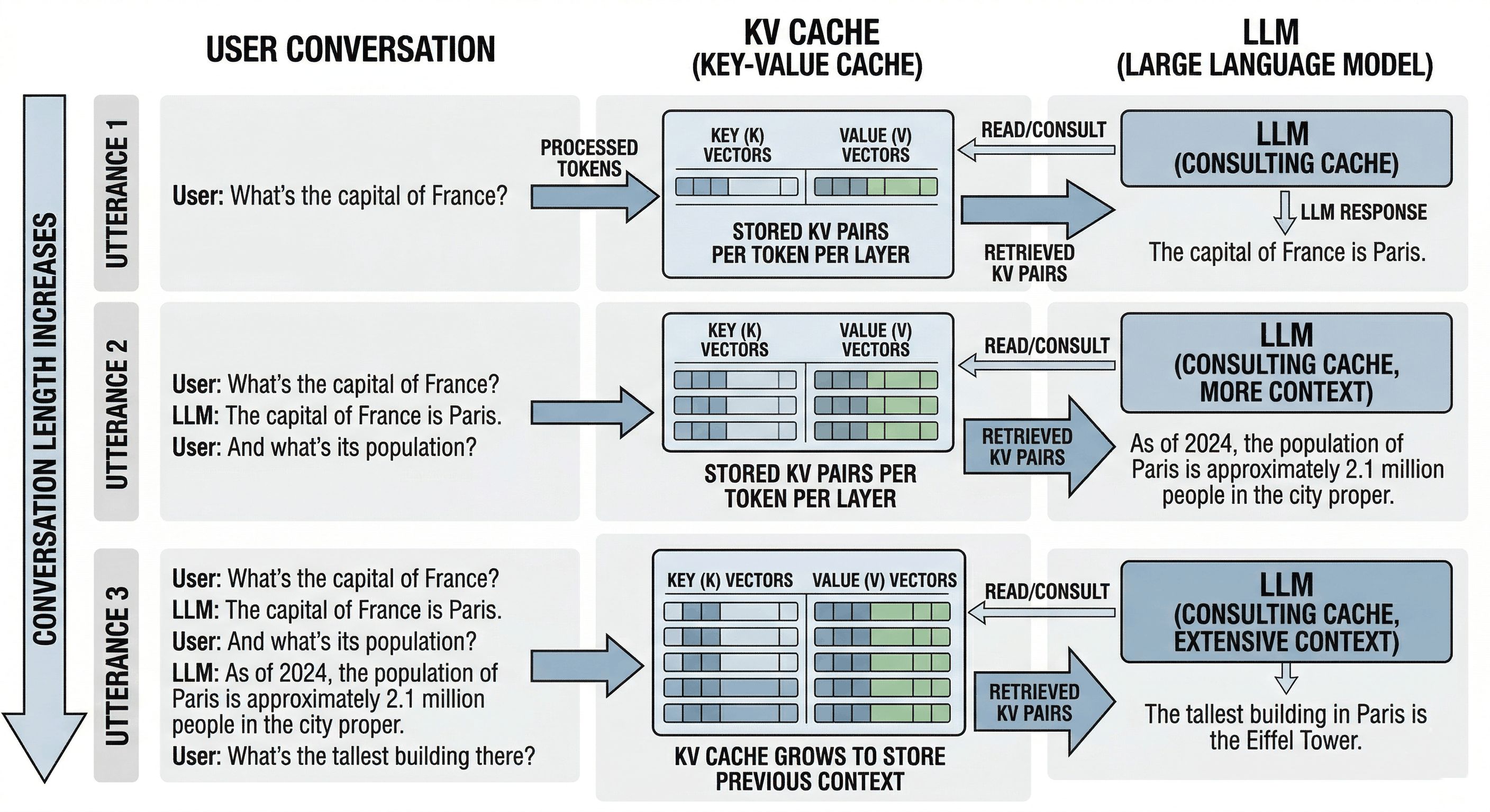
When you send a message to an AI chatbot (ChatGPT, Claude, Gemini, take your pick) something you probably don’t think about is happening behind the scenes. The model isn’t just “thinking” about your latest message. It’s re-reading everything you’ve ever said in this conversation, every single time, to figure out what to say next.
That’s expensive. So engineers invented a trick: instead of re-reading your entire conversation each turn, the model computes a set of summary vectors for every token (word/subword) it has seen and caches them. This is called the KV cache, short for Key-Value cache. Think of it as the model’s working memory, or more precisely, its cheat sheet: a running set of compressed notes on “who said what, and what did it mean?”
It’s clever. It’s also enormous.
Here’s the brutal arithmetic. Take Llama 70B, a large but widely-used open-source model. Run a long conversation of around 100,000 tokens (not unusual for agentic workflows or document analysis). The KV cache for that single user session consumes roughly 40 GB of GPU memory. An H100 GPU, the crown jewel of Nvidia’s data center lineup at around $30,000, has 80 GB of HBM3 memory total. That means one user’s conversation chews through half a flagship GPU chip.
And that’s before the model’s own weights, which for a 70B-parameter model require another 35-70 GB depending on precision. You can see where this is going. The KV cache isn’t just a cost center. It’s often the primary reason you can’t fit more users, longer contexts, or bigger models onto the hardware you have.
This is what engineers mean when they talk about the “memory wall.” You can have the fastest GPUs in the world and still be stuck waiting on memory bandwidth. As one engineer put it in an online thread: “The real AI bottleneck is often not the model. It is the memory wall.”
The scale that makes this matter
AI inference, which means actually running models for real users as opposed to training them, now accounts for 55% of all AI compute spending. Hyperscalers are pouring nearly $700 billion into AI infrastructure in 2026. The KV cache sits right at the top of the memory bottleneck in all of that.
At cloud rates of $2-3 per hour per H100 GPU, the KV cache is often the difference between profitable and unprofitable AI deployment. When GPU memory fills up with KV caches, the system literally cannot take on new users. You either evict older conversations (losing context) or spin up more hardware (losing money).
6x compression on the KV cache means the same hardware handles roughly 6x more simultaneous conversations. Or 6x longer context windows. Or some mix of both. This is not a minor efficiency tweak; it’s a structural shift in the unit economics of serving AI at scale.
Wait, wasn’t this already solved?
Sort of. Quantization, the practice of rounding model weights or activations from high-precision floats (16-bit or 32-bit) to lower-precision integers (8-bit, 4-bit), has been around for years. You’ve probably seen tools like GPTQ, AWQ, or llama.cpp’s GGUF format. These all compress model weights to make them fit on consumer hardware.
But there’s a subtle and important distinction: TurboQuant doesn’t touch model weights at all. It compresses the KV cache, the intermediate attention scores computed fresh at inference time, not the static parameters. The practical consequence is significant: you can run a 4-bit quantized Llama model and then apply TurboQuant on top, getting compression benefits from both independently. They’re not competing; they’re complementary.
Previous KV cache quantization methods (the leading baseline is called KIVI) also tried to quantize the cache, but they introduced their own memory overhead by needing to store quantization constants alongside the compressed data, which partially undermined the savings. TurboQuant’s core innovation is eliminating that overhead almost entirely.
The math is beautiful (even if you hated linear algebra)
Here’s where it gets genuinely elegant. The specific theorem at the heart of this algorithm is the Johnson-Lindenstrauss Lemma, proved in 1984.
The JL Lemma says something remarkable: you can take a set of n points in high-dimensional space and project them down to a much lower-dimensional space (roughly proportional to log(n)) while preserving the pairwise distances between those points. You don’t lose the geometry; you just fold it into a smaller container.
This isn’t just a nice theoretical curiosity. It’s the mathematical foundation for why random projections (multiplying your data by a random matrix) don’t destroy the structure of your information. The structure is preserved in expectation, provably, with quantifiable error bounds.
Before we get to how TurboQuant uses this, let’s make sure the core mechanics of quantization itself are clear, because the intuition matters and it’s simpler than most explanations make it sound.
Quantization in plain English: it’s just putting numbers in bins
At its heart, quantization is about putting data into “bins” so you can represent it with fewer bits. Think of it like rounding: 3.14159 becomes 3. The challenge is that some datasets have wildly uneven distributions that make bin assignment wasteful.
Consider a concrete example. Take this set of numbers: [3.11, 4.43, 5.78, 12.33, 34.32]. Using a simple floor function, these map to [3, 4, 5, 12, 34]. The problem is the outlier: that single value at 34.32 forces you to use 6 bits of information to cover the full range (since 2^6 = 64), even though four of your five values are tightly clustered between 3 and 6. Most of your bit budget is being spent on a single outlier.
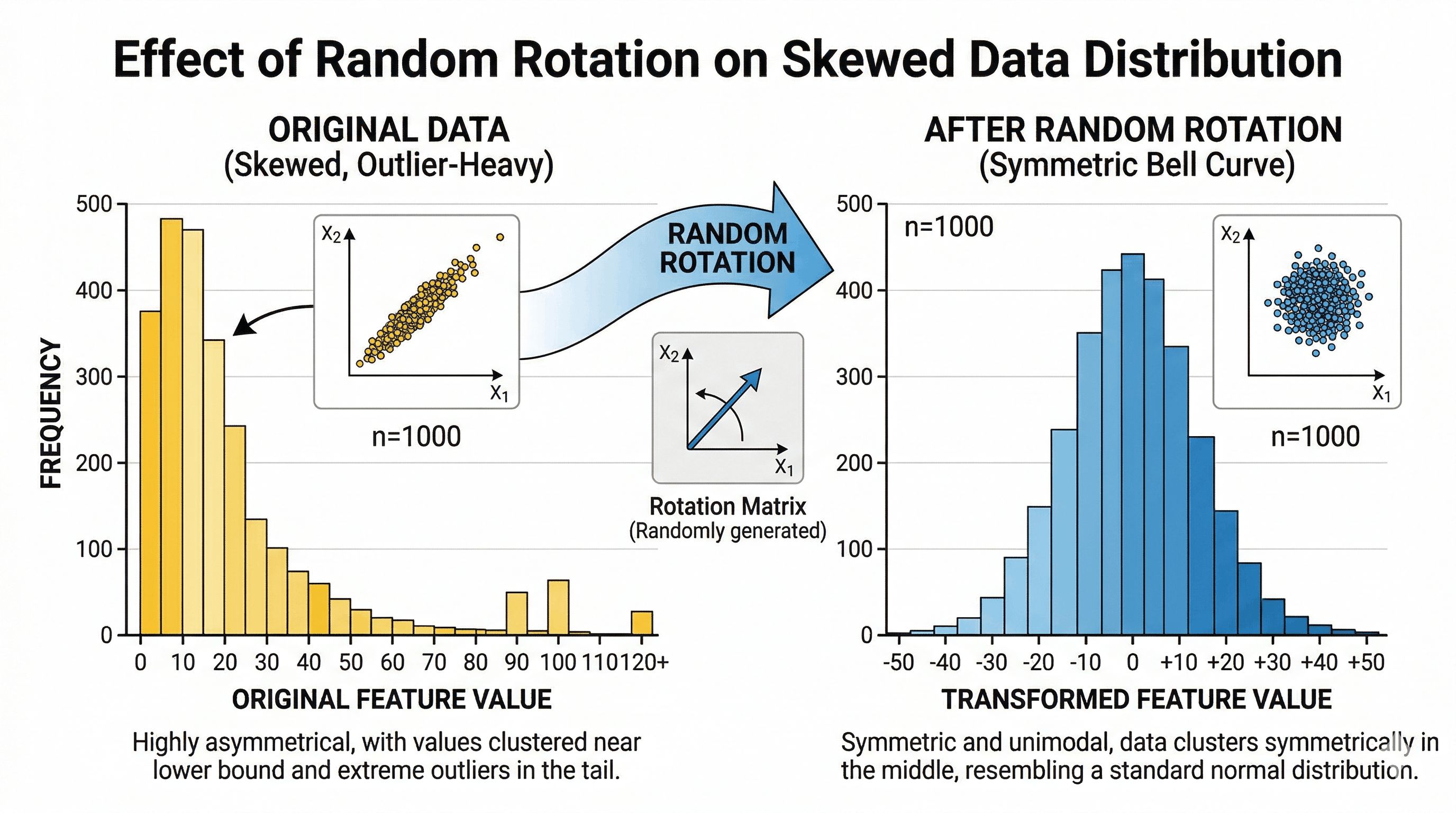
This is exactly the problem random rotation solves. A rotation matrix is an orthogonal matrix in linear algebra terms: when you multiply your vector by it, you aren’t changing the “amount” of data (the vector length stays the same), but you are recalculating every single number as a weighted sum of the originals. By the Central Limit Theorem, when you sum up many random things, the result starts looking like a bell curve.
TurboQuant relies on exactly this: it doesn’t know what your data looks like, but it does know that after the random rotation, the coordinates must follow a predictable Beta distribution (well-approximated by a bell curve). After that rotation, the original [3.11, 4.43, 5.78, 12.33, 34.32] might become something like [8.12, 8.65, 9.25, 10.53, 12.86]: tightly packed, predictably distributed, no outliers. Now your bins can be placed tightly around that bell curve shape, giving you much higher precision with far fewer bits.
To find the most optimal bin placement, TurboQuant uses the Lloyd-Max algorithm, the gold standard for 1D quantization, which finds the best boundaries and reconstruction values to minimize mean squared error.
Why that’s not quite enough, and what fixes it
After Lloyd-Max quantization, you have compressed data, but there’s still a small residual error. In isolation it looks negligible. The problem is that the attention mechanism in transformers is built entirely on dot products (inner products) between query and key vectors. Small quantization errors introduce a bias that accumulates as dot products are computed across long sequences. Left uncorrected, this compounds into real degradation at 100,000+ token context lengths.
The QJL stage is the error-correction step. It takes the quantization residual (the leftover error after step 1) and encodes it using just 1 bit per dimension. That single bit doesn’t represent the original data; it represents the bias introduced by quantization, and it’s enough to mathematically cancel out all the accumulated bias in the dot product estimates.
The way to think about it: it’s a “1-bit note” that allows you to perfectly cancel out all the bias terms your quantization algorithm produces, making the interactions (inner products) extremely accurate again even after compressing the original data. The key insight is that high reconstruction error is fine, because TurboQuant doesn’t need accurate vector reconstruction. It needs accurate attention scores. The QJL correction ensures those are unbiased with variance proportional to 1/d, where d is the head dimension (typically 128). The model’s attention distribution over tokens is preserved even when individual vectors look quite different from their originals.
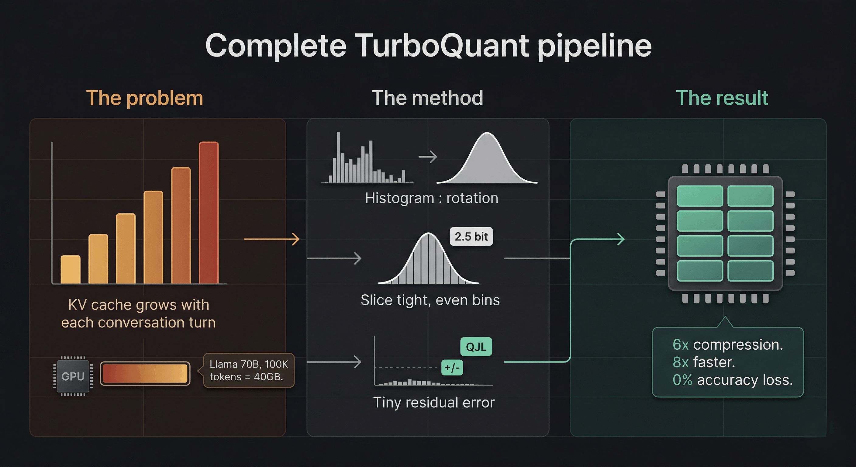
How TurboQuant actually works: the full pipeline
Now that the intuitions are in place, here’s the complete architecture in four steps:
Step 1: Random rotation (change of basis)
Each KV vector gets multiplied by a random orthogonal matrix: a random rotation in high-dimensional space. This preserves dot products (critical for attention), transforms coordinates into a predictable bell-curve distribution, and eliminates the outlier problem. Bins can now be placed optimally.
Step 2: PolarQuant compression (most of the bits)
Rather than quantizing in standard Cartesian coordinates, PolarQuant converts vectors into polar coordinates: each pair of values is represented as a radius (how strong is the signal?) and an angle (what direction is it pointing?). After the rotation step, these angles follow a highly predictable distribution on a fixed circular grid. The quantizer doesn’t need to dynamically figure out the boundaries; they’re already known. This is how PolarQuant eliminates the memory overhead that plagued earlier methods. This stage uses most of the available bits (roughly 2.5 bits of a 3.5-bit total budget) to capture the main signal.
Step 3: QJL residual correction (1 bit)
The Quantized Johnson-Lindenstrauss transform takes the residual error from step 2, projects it through a random Gaussian matrix, and stores just the sign (+1 or -1) of each projection. Exactly 1 bit per dimension. This is enough, provably, to produce an unbiased dot product estimate. The combined inner product estimator is:
<q, k> ≈ <q, k_stage1> + ||residual|| × √(π/2)/m × <S·q, sign(S·residual)>
The first term is the coarse approximation. The second term is the 1-bit stochastic correction. Together they cancel the accumulated bias with zero memory overhead from normalization constants.
Step 4: Fast GPU execution
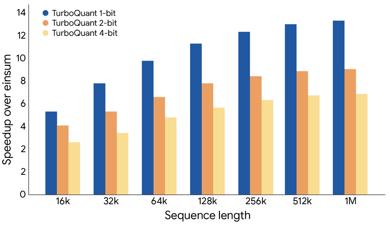
TurboQuant is specifically engineered around the Hadamard transform, which GPUs execute extremely efficiently. On H100 accelerators, 4-bit TurboQuant achieves up to 8x speedup in computing attention logits compared to 32-bit uncompressed keys. Not just less memory: actually faster.
What the numbers actually look like
A community PyTorch implementation validated the paper’s claims on real hardware (RTX 3060, Qwen2.5-3B-Instruct):
| Configuration | KV cache size (8K context) | Compression |
|---|---|---|
| FP16 baseline | 289 MB | 1.0x |
| TurboQuant 4-bit | 76 MB | 3.8x |
| TurboQuant 3-bit | 58 MB | 5.0x |
| TurboQuant 2-bit | 40 MB | 7.3x |
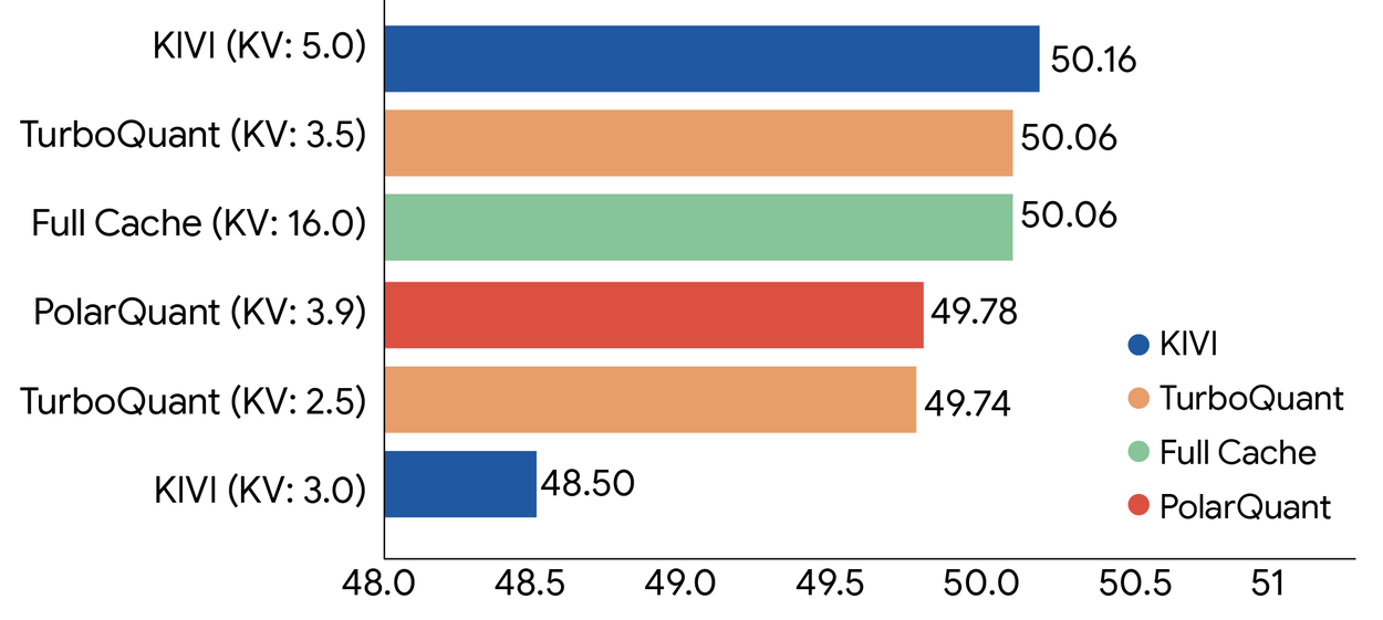
More importantly, the accuracy of attention scores at 3-bit, measured as cosine similarity between compressed and original attention patterns, comes in at 0.9945-0.9961: essentially 99.5% fidelity. The model sees the same tokens, in essentially the same order of importance, that it would have seen with full precision.
The 3-bit configuration is the practical sweet spot: 5x compression, 99.5% attention fidelity. At 2-bit you start seeing degradation in which tokens the model attends to. At 3.5 bits, the paper claims near-lossless results across all tested benchmarks, including perfect scores on Needle-in-a-Haystack tests across context lengths up to 104,000 tokens. That benchmark, finding one specific fact buried deep in a massive document, is the most direct proxy for whether TurboQuant makes the model forget things. It doesn’t.
The real-world impact: from data centers to your desk
For the hyperscalers (Google, Microsoft, Amazon and friends): 6x KV cache compression translates to 6x more users per GPU, or 6x longer context windows for the same hardware bill. At $2-3 per GPU-hour and billions of API calls per day, this is a nine-figure annual savings number. The arXiv preprint came out in April 2025, a full year before the public blog post. The biggest labs have almost certainly been using TurboQuant-class techniques internally for a while.
For the AI inference startup ecosystem: The unit economics just shifted structurally. If you can run a 70B model locally with reasonable latency, you stop paying for cloud API subscriptions and start building a private, local-first stack. The moat of mid-tier SaaS wrappers around foundation models just got meaningfully thinner.
For local AI enthusiasts: This is genuinely transformative. Top-tier models in the 128B parameter range could theoretically run at full quality on 128 GB of RAM, the kind of configuration available in a maxed-out Mac Studio or a well-equipped workstation. With TurboQuant stacked on top of 4-bit weight quantization, the gap between “local open-source AI” and “$200/month cloud subscription” just got meaningfully smaller.
For vector search: TurboQuant isn’t only a KV cache trick. It also works as a standalone improvement to vector similarity search, the technology that powers how search engines and recommendation systems find similar items across billions of entries. Google runs billions of these searches daily. TurboQuant outperforms state-of-the-art baselines on recall benchmarks while requiring no dataset-specific tuning or large codebooks. Same algorithm, two massive application areas.
A note on prior art: the question the research community raised
Not everyone was purely celebratory. In technical discussions, a researcher flagged something worth paying attention to: the foundational technique of applying a geometric rotation prior to extreme quantization, specifically for managing high-dimensional geometry and enabling proper bias correction, was introduced in a NeurIPS 2021 paper called DRIVE, which tackled optimal distributed mean estimation using exactly this rotational approach and a similar bias correction mechanism. The researcher noted having presented this work in a private invited talk at Google shortly after publication, and expressed hope that the camera-ready version of the TurboQuant paper would acknowledge this prior art.
The discussion that followed was illuminating. When someone asked whether the “rotation” was essentially diagonalization (storing a diagonal matrix plus new basis vectors for compactness), the response clarified: not quite. The rotation isn’t about finding a compact diagonal representation. Its purpose is to spread energy across dimensions and ensure predictable coordinate distributions, making coordinate-wise quantization computationally efficient. The trade-off is that it throws away any learnable structure in the original vectors. As someone in the thread summarized: “Intuitively it’s like minimizing the error when replacing values with a well-known distribution. All you need to carry along is the rotation and the assumption that there is some amount of loss.”
This is worth flagging for two reasons. First, attribution matters in research, and the community is right to expect it. Second, it underscores the power of the underlying idea: the rotation-then-quantize paradigm was independently useful enough that multiple research groups converged on it from different directions.
The question everyone keeps asking: why did Google just give this away?
When a company with Google’s resources publishes an algorithm that could reshape the economics of the entire AI industry, people get suspicious. The discussions in online communities clustered around a few theories:
Theory 1: They already have something better. Probably the safest assumption. The arXiv preprint is from April 2025, a full year before the blog post. Publishing it now gets credit and goodwill without revealing the actual current state of internal tooling.
Theory 2: Talent acquisition. Top ML researchers won’t join a company where they can’t publish. Letting researchers publish, even work that includes valuable techniques, is often a better trade than the attrition that comes from not letting them.
Theory 3: Ecosystem pressure on memory. If TurboQuant reduces industry-wide demand for high-bandwidth memory, HBM prices moderate. Google runs its own TPU infrastructure, designed in-house. Reducing the whole industry’s memory pressure has asymmetric benefits for vertically integrated compute players.
Theory 4: It’s just how science works. Google Research has a long history of publishing foundational work, including “Attention Is All You Need,” the Transformer paper that spawned the entire current LLM era. Sometimes researchers at well-resourced companies genuinely want to share what they figured out. As one commenter put it: “If there is one overwhelming instinct in tech folk, one constantly in conflict with the business side, it is the desire to share the latest clever idea.”
All four theories are probably partially true. The most honest answer is that ideas like TurboQuant are genuinely not rare enough to hoard for long. Given similar incentives and the same mathematical foundations, other labs were converging on similar conclusions. Getting there first, in public, is worth more as a reputational and recruiting asset than as a kept secret.
Try it yourself
A clean from-scratch PyTorch implementation is available at tonbistudio/turboquant-pytorch. It includes a synthetic validation suite that tests the algorithm against the paper’s theoretical bounds, a real model validation script using Qwen2.5-3B-Instruct that you can run on any CUDA GPU with at least 6 GB VRAM, and readable implementations of all three components: Lloyd-Max codebook solver, TurboQuant MSE stage, and QJL residual correction.
Community implementations are already appearing in MLX for Apple Silicon, and it’s a matter of time before this lands in vLLM, llama.cpp, and the other major inference frameworks.
For the more visually inclined, someone turned the paper into an interactive Marimo notebook where you can drag sliders and watch the math happen in real time, exploring how random rotations, Beta distributions, and quantization interact. It’s the best way to build intuition before diving into the code.
The part nobody is pricing in
TurboQuant is a systems innovation, not a model innovation. It doesn’t make the underlying model smarter. It makes the memory required to run a smart model dramatically smaller. And this category of innovation (inference efficiency, memory compression, hardware-software co-design) is where a disproportionate share of real-world AI progress is happening right now, mostly out of the spotlight.
The benchmark numbers are clean. Production is always messier: adversarial inputs, unusual token distributions, edge cases the paper didn’t test. The “zero accuracy loss” claim deserves healthy skepticism at scale. But the theoretical foundations here are solid. These results are provably near theoretical lower bounds for distortion, not just empirically observed on a handful of benchmarks.
And this is not an isolated breakthrough. It’s one piece of a larger picture in which better quantization, smarter memory management, more efficient attention mechanisms, and cheaper hardware are all improving simultaneously. The open-source models available today on consumer hardware are genuinely capable. The hardware you already own is meaningfully more powerful than it was 12 months ago. The trajectory is clear, and it’s accelerating.
Closing thought
The fictional Pied Piper algorithm was a joke about Silicon Valley hubris: a solution looking for a problem, run by founders who couldn’t quite grasp what they’d built.
TurboQuant is the opposite story. Researchers who knew exactly what problem they were solving, grounded the solution in 40-year-old mathematics, proved it rigorously, tested it on real hardware, and then gave it away. Not because they had to. Because that’s what you do with good science.
The KV cache is the most expensive cheat sheet in the history of computing. It just got a lot cheaper.
Sources: